Exploratory Data Analysis#
EDA is the process of performing initial investigations on data to discover patterns, spot anomalies, test hypothesis and check assumptions.
EDA is important for the following reasons, it helps to:
Understand the data better.
Identify the outliers.
Identify the missing values.
Relationship between variables.
Normality of the data.
Outliers.
Correlation between variables.
Distribution of the data. etc.
To start with EDA, we need to understand the problem statement.
Understand the problem. We’ll look at each variable and do a philosophical analysis about their meaning and importance for this problem.
Univariable study. We’ll just focus on the dependent variable (‘SalePrice’) and try to know a little bit more about it.
Multivariate study. We’ll try to understand how the dependent variable and independent variables relate.
Basic cleaning. We’ll clean the dataset and handle the missing data, outliers and categorical variables.
Test assumptions. We’ll check if our data meets the assumptions required by most multivariate techniques.
Now, it’s time to have fun!
import pandas as pd
import matplotlib.pyplot as plt
import seaborn as sns
import numpy as np
from scipy.stats import norm
from sklearn.preprocessing import StandardScaler
from scipy import stats
import warnings
warnings.filterwarnings('ignore')
%matplotlib inline
About the dataset
The dataset we’ll use is the well-known Ames Housing dataset. It is a dataset with 81 variables. The goal is to predict the price of a house based on its features.
The dataset is available on Kaggle.
To understand the description of the columns in teh dataset, lets load house_price_data_description.txt file.
# read teh data description file
with open('house_price_data_description.txt', 'r') as file:
    print(file.read())
MSSubClass: Identifies the type of dwelling involved in the sale.

        20	1-STORY 1946 & NEWER ALL STYLES
        30	1-STORY 1945 & OLDER
        40	1-STORY W/FINISHED ATTIC ALL AGES
        45	1-1/2 STORY - UNFINISHED ALL AGES
        50	1-1/2 STORY FINISHED ALL AGES
        60	2-STORY 1946 & NEWER
        70	2-STORY 1945 & OLDER
        75	2-1/2 STORY ALL AGES
        80	SPLIT OR MULTI-LEVEL
        85	SPLIT FOYER
        90	DUPLEX - ALL STYLES AND AGES
       120	1-STORY PUD (Planned Unit Development) - 1946 & NEWER
       150	1-1/2 STORY PUD - ALL AGES
       160	2-STORY PUD - 1946 & NEWER
       180	PUD - MULTILEVEL - INCL SPLIT LEV/FOYER
       190	2 FAMILY CONVERSION - ALL STYLES AND AGES

MSZoning: Identifies the general zoning classification of the sale.

       A	Agriculture
       C	Commercial
       FV	Floating Village Residential
       I	Industrial
       RH	Residential High Density
       RL	Residential Low Density
       RP	Residential Low Density Park
       RM	Residential Medium Density

LotFrontage: Linear feet of street connected to property

LotArea: Lot size in square feet

Street: Type of road access to property

       Grvl	Gravel
       Pave	Paved

Alley: Type of alley access to property

       Grvl	Gravel
       Pave	Paved
       NA 	No alley access

LotShape: General shape of property

       Reg	Regular
       IR1	Slightly irregular
       IR2	Moderately Irregular
       IR3	Irregular

LandContour: Flatness of the property

       Lvl	Near Flat/Level
       Bnk	Banked - Quick and significant rise from street grade to building
       HLS	Hillside - Significant slope from side to side
       Low	Depression

Utilities: Type of utilities available

       AllPub	All public Utilities (E,G,W,& S)
       NoSewr	Electricity, Gas, and Water (Septic Tank)
       NoSeWa	Electricity and Gas Only
       ELO	Electricity only

LotConfig: Lot configuration

       Inside	Inside lot
       Corner	Corner lot
       CulDSac	Cul-de-sac
       FR2	Frontage on 2 sides of property
       FR3	Frontage on 3 sides of property

LandSlope: Slope of property

       Gtl	Gentle slope
       Mod	Moderate Slope
       Sev	Severe Slope

Neighborhood: Physical locations within Ames city limits

       Blmngtn	Bloomington Heights
       Blueste	Bluestem
       BrDale	Briardale
       BrkSide	Brookside
       ClearCr	Clear Creek
       CollgCr	College Creek
       Crawfor	Crawford
       Edwards	Edwards
       Gilbert	Gilbert
       IDOTRR	Iowa DOT and Rail Road
       MeadowV	Meadow Village
       Mitchel	Mitchell
       Names	North Ames
       NoRidge	Northridge
       NPkVill	Northpark Villa
       NridgHt	Northridge Heights
       NWAmes	Northwest Ames
       OldTown	Old Town
       SWISU	South & West of Iowa State University
       Sawyer	Sawyer
       SawyerW	Sawyer West
       Somerst	Somerset
       StoneBr	Stone Brook
       Timber	Timberland
       Veenker	Veenker

Condition1: Proximity to various conditions

       Artery	Adjacent to arterial street
       Feedr	Adjacent to feeder street
       Norm	Normal
       RRNn	Within 200' of North-South Railroad
       RRAn	Adjacent to North-South Railroad
       PosN	Near positive off-site feature--park, greenbelt, etc.
       PosA	Adjacent to postive off-site feature
       RRNe	Within 200' of East-West Railroad
       RRAe	Adjacent to East-West Railroad

Condition2: Proximity to various conditions (if more than one is present)

       Artery	Adjacent to arterial street
       Feedr	Adjacent to feeder street
       Norm	Normal
       RRNn	Within 200' of North-South Railroad
       RRAn	Adjacent to North-South Railroad
       PosN	Near positive off-site feature--park, greenbelt, etc.
       PosA	Adjacent to postive off-site feature
       RRNe	Within 200' of East-West Railroad
       RRAe	Adjacent to East-West Railroad

BldgType: Type of dwelling

       1Fam	Single-family Detached
       2FmCon	Two-family Conversion; originally built as one-family dwelling
       Duplx	Duplex
       TwnhsE	Townhouse End Unit
       TwnhsI	Townhouse Inside Unit

HouseStyle: Style of dwelling

       1Story	One story
       1.5Fin	One and one-half story: 2nd level finished
       1.5Unf	One and one-half story: 2nd level unfinished
       2Story	Two story
       2.5Fin	Two and one-half story: 2nd level finished
       2.5Unf	Two and one-half story: 2nd level unfinished
       SFoyer	Split Foyer
       SLvl	Split Level

OverallQual: Rates the overall material and finish of the house

       10	Very Excellent
       9	Excellent
       8	Very Good
       7	Good
       6	Above Average
       5	Average
       4	Below Average
       3	Fair
       2	Poor
       1	Very Poor

OverallCond: Rates the overall condition of the house

       10	Very Excellent
       9	Excellent
       8	Very Good
       7	Good
       6	Above Average
       5	Average
       4	Below Average
       3	Fair
       2	Poor
       1	Very Poor

YearBuilt: Original construction date

YearRemodAdd: Remodel date (same as construction date if no remodeling or additions)

RoofStyle: Type of roof

       Flat	Flat
       Gable	Gable
       Gambrel	Gabrel (Barn)
       Hip	Hip
       Mansard	Mansard
       Shed	Shed

RoofMatl: Roof material

       ClyTile	Clay or Tile
       CompShg	Standard (Composite) Shingle
       Membran	Membrane
       Metal	Metal
       Roll	Roll
       Tar&Grv	Gravel & Tar
       WdShake	Wood Shakes
       WdShngl	Wood Shingles

Exterior1st: Exterior covering on house

       AsbShng	Asbestos Shingles
       AsphShn	Asphalt Shingles
       BrkComm	Brick Common
       BrkFace	Brick Face
       CBlock	Cinder Block
       CemntBd	Cement Board
       HdBoard	Hard Board
       ImStucc	Imitation Stucco
       MetalSd	Metal Siding
       Other	Other
       Plywood	Plywood
       PreCast	PreCast
       Stone	Stone
       Stucco	Stucco
       VinylSd	Vinyl Siding
       Wd Sdng	Wood Siding
       WdShing	Wood Shingles

Exterior2nd: Exterior covering on house (if more than one material)

       AsbShng	Asbestos Shingles
       AsphShn	Asphalt Shingles
       BrkComm	Brick Common
       BrkFace	Brick Face
       CBlock	Cinder Block
       CemntBd	Cement Board
       HdBoard	Hard Board
       ImStucc	Imitation Stucco
       MetalSd	Metal Siding
       Other	Other
       Plywood	Plywood
       PreCast	PreCast
       Stone	Stone
       Stucco	Stucco
       VinylSd	Vinyl Siding
       Wd Sdng	Wood Siding
       WdShing	Wood Shingles

MasVnrType: Masonry veneer type

       BrkCmn	Brick Common
       BrkFace	Brick Face
       CBlock	Cinder Block
       None	None
       Stone	Stone

MasVnrArea: Masonry veneer area in square feet

ExterQual: Evaluates the quality of the material on the exterior

       Ex	Excellent
       Gd	Good
       TA	Average/Typical
       Fa	Fair
       Po	Poor

ExterCond: Evaluates the present condition of the material on the exterior

       Ex	Excellent
       Gd	Good
       TA	Average/Typical
       Fa	Fair
       Po	Poor

Foundation: Type of foundation

       BrkTil	Brick & Tile
       CBlock	Cinder Block
       PConc	Poured Contrete
       Slab	Slab
       Stone	Stone
       Wood	Wood

BsmtQual: Evaluates the height of the basement

       Ex	Excellent (100+ inches)
       Gd	Good (90-99 inches)
       TA	Typical (80-89 inches)
       Fa	Fair (70-79 inches)
       Po	Poor (<70 inches
       NA	No Basement

BsmtCond: Evaluates the general condition of the basement

       Ex	Excellent
       Gd	Good
       TA	Typical - slight dampness allowed
       Fa	Fair - dampness or some cracking or settling
       Po	Poor - Severe cracking, settling, or wetness
       NA	No Basement

BsmtExposure: Refers to walkout or garden level walls

       Gd	Good Exposure
       Av	Average Exposure (split levels or foyers typically score average or above)
       Mn	Mimimum Exposure
       No	No Exposure
       NA	No Basement

BsmtFinType1: Rating of basement finished area

       GLQ	Good Living Quarters
       ALQ	Average Living Quarters
       BLQ	Below Average Living Quarters
       Rec	Average Rec Room
       LwQ	Low Quality
       Unf	Unfinshed
       NA	No Basement

BsmtFinSF1: Type 1 finished square feet

BsmtFinType2: Rating of basement finished area (if multiple types)

       GLQ	Good Living Quarters
       ALQ	Average Living Quarters
       BLQ	Below Average Living Quarters
       Rec	Average Rec Room
       LwQ	Low Quality
       Unf	Unfinshed
       NA	No Basement

BsmtFinSF2: Type 2 finished square feet

BsmtUnfSF: Unfinished square feet of basement area

TotalBsmtSF: Total square feet of basement area

Heating: Type of heating

       Floor	Floor Furnace
       GasA	Gas forced warm air furnace
       GasW	Gas hot water or steam heat
       Grav	Gravity furnace
       OthW	Hot water or steam heat other than gas
       Wall	Wall furnace

HeatingQC: Heating quality and condition

       Ex	Excellent
       Gd	Good
       TA	Average/Typical
       Fa	Fair
       Po	Poor

CentralAir: Central air conditioning

       N	No
       Y	Yes

Electrical: Electrical system

       SBrkr	Standard Circuit Breakers & Romex
       FuseA	Fuse Box over 60 AMP and all Romex wiring (Average)
       FuseF	60 AMP Fuse Box and mostly Romex wiring (Fair)
       FuseP	60 AMP Fuse Box and mostly knob & tube wiring (poor)
       Mix	Mixed

1stFlrSF: First Floor square feet

2ndFlrSF: Second floor square feet

LowQualFinSF: Low quality finished square feet (all floors)

GrLivArea: Above grade (ground) living area square feet

BsmtFullBath: Basement full bathrooms

BsmtHalfBath: Basement half bathrooms

FullBath: Full bathrooms above grade

HalfBath: Half baths above grade

Bedroom: Bedrooms above grade (does NOT include basement bedrooms)

Kitchen: Kitchens above grade

KitchenQual: Kitchen quality

       Ex	Excellent
       Gd	Good
       TA	Typical/Average
       Fa	Fair
       Po	Poor

TotRmsAbvGrd: Total rooms above grade (does not include bathrooms)

Functional: Home functionality (Assume typical unless deductions are warranted)

       Typ	Typical Functionality
       Min1	Minor Deductions 1
       Min2	Minor Deductions 2
       Mod	Moderate Deductions
       Maj1	Major Deductions 1
       Maj2	Major Deductions 2
       Sev	Severely Damaged
       Sal	Salvage only

Fireplaces: Number of fireplaces

FireplaceQu: Fireplace quality

       Ex	Excellent - Exceptional Masonry Fireplace
       Gd	Good - Masonry Fireplace in main level
       TA	Average - Prefabricated Fireplace in main living area or Masonry Fireplace in basement
       Fa	Fair - Prefabricated Fireplace in basement
       Po	Poor - Ben Franklin Stove
       NA	No Fireplace

GarageType: Garage location

       2Types	More than one type of garage
       Attchd	Attached to home
       Basment	Basement Garage
       BuiltIn	Built-In (Garage part of house - typically has room above garage)
       CarPort	Car Port
       Detchd	Detached from home
       NA	No Garage

GarageYrBlt: Year garage was built

GarageFinish: Interior finish of the garage

       Fin	Finished
       RFn	Rough Finished
       Unf	Unfinished
       NA	No Garage

GarageCars: Size of garage in car capacity

GarageArea: Size of garage in square feet

GarageQual: Garage quality

       Ex	Excellent
       Gd	Good
       TA	Typical/Average
       Fa	Fair
       Po	Poor
       NA	No Garage

GarageCond: Garage condition

       Ex	Excellent
       Gd	Good
       TA	Typical/Average
       Fa	Fair
       Po	Poor
       NA	No Garage

PavedDrive: Paved driveway

       Y	Paved
       P	Partial Pavement
       N	Dirt/Gravel

WoodDeckSF: Wood deck area in square feet

OpenPorchSF: Open porch area in square feet

EnclosedPorch: Enclosed porch area in square feet

3SsnPorch: Three season porch area in square feet

ScreenPorch: Screen porch area in square feet

PoolArea: Pool area in square feet

PoolQC: Pool quality

       Ex	Excellent
       Gd	Good
       TA	Average/Typical
       Fa	Fair
       NA	No Pool

Fence: Fence quality

       GdPrv	Good Privacy
       MnPrv	Minimum Privacy
       GdWo	Good Wood
       MnWw	Minimum Wood/Wire
       NA	No Fence

MiscFeature: Miscellaneous feature not covered in other categories

       Elev	Elevator
       Gar2	2nd Garage (if not described in garage section)
       Othr	Other
       Shed	Shed (over 100 SF)
       TenC	Tennis Court
       NA	None

MiscVal: $Value of miscellaneous feature

MoSold: Month Sold (MM)

YrSold: Year Sold (YYYY)

SaleType: Type of sale

       WD 	Warranty Deed - Conventional
       CWD	Warranty Deed - Cash
       VWD	Warranty Deed - VA Loan
       New	Home just constructed and sold
       COD	Court Officer Deed/Estate
       Con	Contract 15% Down payment regular terms
       ConLw	Contract Low Down payment and low interest
       ConLI	Contract Low Interest
       ConLD	Contract Low Down
       Oth	Other

SaleCondition: Condition of sale

       Normal	Normal Sale
       Abnorml	Abnormal Sale -  trade, foreclosure, short sale
       AdjLand	Adjoining Land Purchase
       Alloca	Allocation - two linked properties with separate deeds, typically condo with a garage unit
       Family	Sale between family members
       Partial	Home was not completed when last assessed (associated with New Homes)
# Let's load the house prices dataset
df_train = pd.read_csv('house_prices.csv')
#check the decoration
df_train.columns
Index(['Id', 'MSSubClass', 'MSZoning', 'LotFrontage', 'LotArea', 'Street',
       'Alley', 'LotShape', 'LandContour', 'Utilities', 'LotConfig',
       'LandSlope', 'Neighborhood', 'Condition1', 'Condition2', 'BldgType',
       'HouseStyle', 'OverallQual', 'OverallCond', 'YearBuilt', 'YearRemodAdd',
       'RoofStyle', 'RoofMatl', 'Exterior1st', 'Exterior2nd', 'MasVnrType',
       'MasVnrArea', 'ExterQual', 'ExterCond', 'Foundation', 'BsmtQual',
       'BsmtCond', 'BsmtExposure', 'BsmtFinType1', 'BsmtFinSF1',
       'BsmtFinType2', 'BsmtFinSF2', 'BsmtUnfSF', 'TotalBsmtSF', 'Heating',
       'HeatingQC', 'CentralAir', 'Electrical', '1stFlrSF', '2ndFlrSF',
       'LowQualFinSF', 'GrLivArea', 'BsmtFullBath', 'BsmtHalfBath', 'FullBath',
       'HalfBath', 'BedroomAbvGr', 'KitchenAbvGr', 'KitchenQual',
       'TotRmsAbvGrd', 'Functional', 'Fireplaces', 'FireplaceQu', 'GarageType',
       'GarageYrBlt', 'GarageFinish', 'GarageCars', 'GarageArea', 'GarageQual',
       'GarageCond', 'PavedDrive', 'WoodDeckSF', 'OpenPorchSF',
       'EnclosedPorch', '3SsnPorch', 'ScreenPorch', 'PoolArea', 'PoolQC',
       'Fence', 'MiscFeature', 'MiscVal', 'MoSold', 'YrSold', 'SaleType',
       'SaleCondition', 'SalePrice'],
      dtype='object')
Understand the data#
In order to understand our data, we can look at each variable and try to understand their meaning and relevance to this problem.
It is time-consuming, but it will give us the flavour of our dataset.
In order to have some discipline in our analysis, we can create an Excel spreadsheet with the following columns:
Variable - Variable name.
Type - Identification of the variables’ type. There are two possible values for this field: ‘numerical’ or ‘categorical’. By ‘numerical’ we mean variables for which the values are numbers, and by ‘categorical’ we mean variables for which the values are categories.
Segment - Identification of the variables’ segment. We can define three possible segments: building, space or location. When we say ‘building’, we mean a variable that relates to the physical characteristics of the building (e.g. ‘OverallQual’). When we say ‘space’, we mean a variable that reports space properties of the house (e.g. ‘TotalBsmtSF’). Finally, when we say a ‘location’, we mean a variable that gives information about the place where the house is located (e.g. ‘Neighborhood’).
Expectation - Our expectation about the variable influence in ‘SalePrice’. We can use a categorical scale with ‘High’, ‘Medium’ and ‘Low’ as possible values.
Conclusion - Our conclusions about the importance of the variable, after we give a quick look at the data. We can keep with the same categorical scale as in ‘Expectation’.
Comments - Any general comments that occured to us.
While ‘Type’ and ‘Segment’ is just for possible future reference, the column ‘Expectation’ is important because it will help us develop a ‘sixth sense’. To fill this column, we should read the description of all the variables and, one by one, ask ourselves:
Do we think about this variable when we are buying a house? (e.g. When we think about the house of our dreams, do we care about its ‘Masonry veneer type’?).
If so, how important would this variable be? (e.g. What is the impact of having ‘Excellent’ material on the exterior instead of ‘Poor’? And of having ‘Excellent’ instead of ‘Good’?).
Is this information already described in any other variable? (e.g. If ‘LandContour’ gives the flatness of the property, do we really need to know the ‘LandSlope’?).
After this daunting exercise, we can filter the spreadsheet and look carefully to the variables with ‘High’ ‘Expectation’. Then, we can rush into some scatter plots between those variables and ‘SalePrice’, filling in the ‘Conclusion’ column which is just the correction of our expectations.
I went through this process and concluded that the following variables can play an important role in this problem:
OverallQual
YearBuilt.
TotalBsmtSF.
GrLivArea.
I ended up with two ‘building’ variables (‘OverallQual’ and ‘YearBuilt’) and two ‘space’ variables (‘TotalBsmtSF’ and ‘GrLivArea’).
This might be a little bit unexpected as it goes against the real estate mantra that all that matters is ‘location, location and location’.
It is possible that this quick data examination process was a bit harsh for categorical variables. For example, I expected the ‘Neigborhood’ variable to be more relevant, but after the data examination I ended up excluding it. Maybe this is related to the use of scatter plots instead of boxplots, which are more suitable for categorical variables visualization. The way we visualize data often influences our conclusions.
However, the main point of this exercise was to think a little about our data and expectactions, so I think we achieved our goal. Now it’s time for ‘a little less conversation, a little more action please’. Let’s shake it!
Subjective analysis#
‘SalePrice’ is the reason of our quest. first we will do some descriptive analysis, which will help us to understand the distribution of the data
#descriptive statistics summary
df_train['SalePrice'].describe()
count      1460.000000
mean     180921.195890
std       79442.502883
min       34900.000000
25%      129975.000000
50%      163000.000000
75%      214000.000000
max      755000.000000
Name: SalePrice, dtype: float64
#histogram
sns.distplot(df_train['SalePrice']);
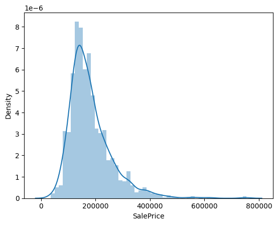
From above plot we can see that:
Deviate from the normal distribution.
Have appreciable positive skewness.
Show peakedness.
Skewness and kurtosis
Skewness is a measure of the asymmetry of the data distribution. It tells us about the direction of the outliers. If the skewness is negative, the tail is on the left side of the distribution and if it is positive, the tail is on the right side.
Kurtosis is a measure of the “tailedness” of the data distribution. It tells us about the outliers of the data distribution. If the kurtosis is high, the data distribution has heavy tails and the outliers are more spread out. If the kurtosis is low, the data distribution has light tails and the outliers are more concentrated.
Skewness and kurtosis are important because they help us understand the shape of the data distribution and the presence of outliers.
#skewness and kurtosis
print("Skewness: %f" % df_train['SalePrice'].skew())
print("Kurtosis: %f" % df_train['SalePrice'].kurt())
Skewness: 1.882876
Kurtosis: 6.536282
What does the abovve number mean?
Skewness: 1.882876
Kurtosis: 6.529276
A value of 0 indicates a normal distribution,
while positive values indicate a right-skewed distribution and
negative values indicate a left-skewed distribution.
In this case, the skewness value of 1.882876 indicates that the ‘SalePrice’ distribution is moderately right-skewed. This means that there are more values on the left side of the distribution and fewer values on the right side.
The kurtosis value of 6.529276 indicates that the distribution is more peaked (leptokurtic) than a normal distribution, which suggests the presence of outliers or extreme values in the data.
Releationship of ‘SalePrice’ with other variables#
Relationship with numerical variables#
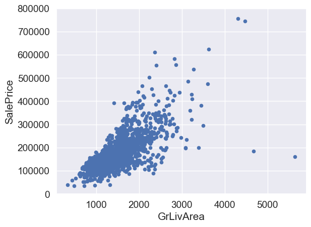
#scatter plot grlivarea/saleprice
var = 'GrLivArea'
data = pd.concat([df_train['SalePrice'], df_train[var]], axis=1)
data.plot.scatter(x=var, y='SalePrice', ylim=(0,800000));
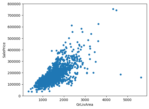
‘SalePrice’ and ‘GrLivArea’ follow a linear relationship.
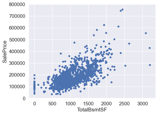
Let’s check the relationship between ‘SalePrice’ and ‘TotalBsmtSF’.
#scatter plot totalbsmtsf/saleprice
var = 'TotalBsmtSF'
data = pd.concat([df_train['SalePrice'], df_train[var]], axis=1)
data.plot.scatter(x=var, y='SalePrice', ylim=(0,800000));
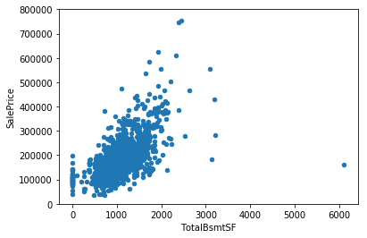
‘TotalBsmtSF’ also has a strong relationship with ‘SalePrice’ which can be an exponential or a strong linear relationship.
Relationship with categorical features#
#box plot overallqual/saleprice
var = 'OverallQual'
data = pd.concat([df_train['SalePrice'], df_train[var]], axis=1)
f, ax = plt.subplots(figsize=(8, 6))
fig = sns.boxplot(x=var, y="SalePrice", data=data)
fig.axis(ymin=0, ymax=800000);
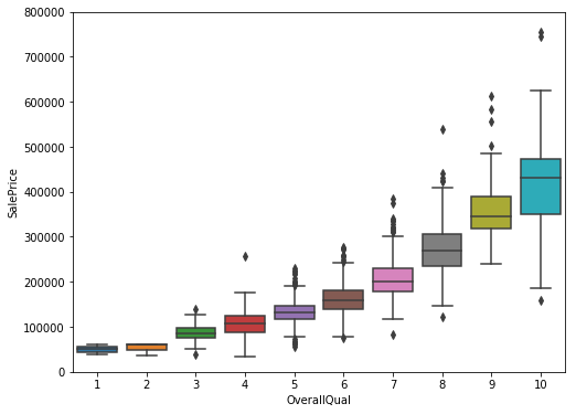
Above plot shows that as the Overall quality of the house increases as the Sale price increases, which makes sense.
The box plot is a good way to compare the distribution of the Sale price for different levels of Overall quality.
Let’s do the same for ‘YearBuilt’
var = 'YearBuilt'
data = pd.concat([df_train['SalePrice'], df_train[var]], axis=1)
f, ax = plt.subplots(figsize=(16, 8))
fig = sns.boxplot(x=var, y="SalePrice", data=data)
fig.axis(ymin=0, ymax=800000);
plt.xticks(rotation=90);
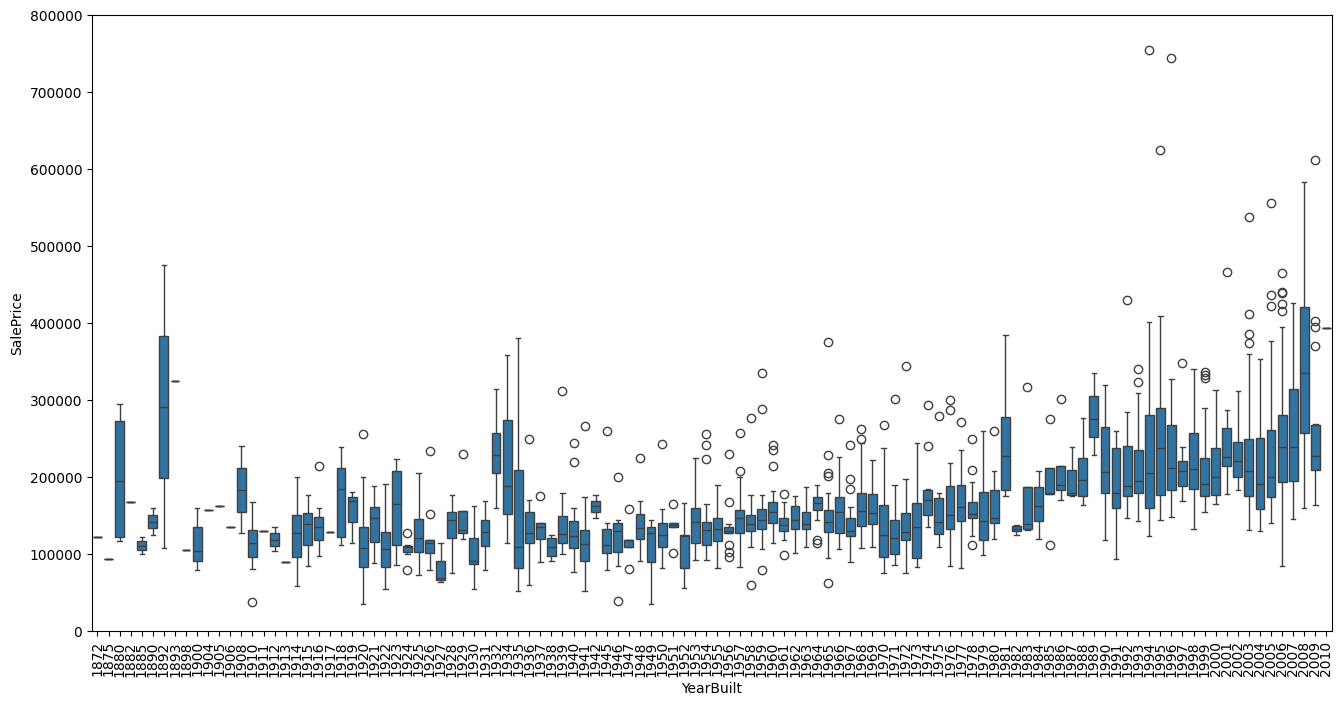
Although not strongly but ‘SalePrice’ is more prone to spend more money in new stuff than in old relics.
Note: we don’t know if ‘SalePrice’ is in constant prices. Constant prices try to remove the effect of inflation. If ‘SalePrice’ is not in constant prices, it should be, so than prices are comparable over the years.
In summary#
Here ,we can conclude that:
‘GrLivArea’ and ‘TotalBsmtSF’ seem to be linearly related with ‘SalePrice’. Both relationships are positive, which means that as one variable increases, the other also increases.
In the case of ‘TotalBsmtSF’, we can see that the slope of the linear relationship is particularly high.
‘OverallQual’ and ‘YearBuilt’ also seem to be related with ‘SalePrice’. The relationship seems to be stronger in the case of ‘OverallQual’, where the box plot shows how sales prices increase with the overall quality.
We just analysed four variables, but there are many other that we should analyse. The trick here seems to be the choice of the right features (feature selection) and not the definition of complex relationships between them (feature engineering).
Objective analysis#
Until now we just followed our intuition and analysed the variables we thought were important. In spite of our efforts to give an objective character to our analysis, we must say that our starting point was subjective.
So, let’s overcome inertia and do a more objective analysis.
Correlation analysis#
To understand the relationship objectively for all sort of variables, we can do some correlation analysis.
Correlation matrix (heatmap style).
‘SalePrice’ correlation matrix (zoomed heatmap style).
Scatter plots between the most correlated variables (move like Jagger style).
Correlation matrix (heatmap style)#
#correlation matrix
numeric_features = df_train.select_dtypes(include=[np.number]).columns
corrmat = df_train[numeric_features].corr()
f, ax = plt.subplots(figsize=(12, 9))
sns.heatmap(corrmat, vmax=.8, square=True)
<Axes: >
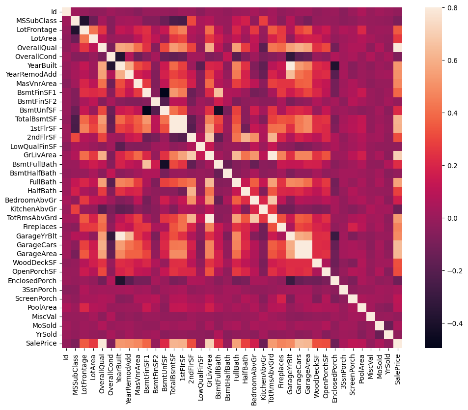
Heatmap is the best way to get a quick overview of the correlation matrix for all the variables.
At first sight, there are two red colored squares that get my attention.
The first one refers to the ‘TotalBsmtSF’ and ‘1stFlrSF’ variables, and
‘GarageX’ variables.
Both cases show how significant the correlation is between these variables. Actually, this correlation is so strong that it can indicate a situation of multicollinearity.
If we think about these variables, we can conclude that they give almost the same information so multicollinearity really occurs.
Heatmaps are great to detect this kind of situations and in problems dominated by feature selection, like ours, they are an essential tool.
Another thing that got my attention was the ‘SalePrice’ correlations. We can see our well-known ‘GrLivArea’, ‘TotalBsmtSF’, and ‘OverallQual’,
But we can also see many other variables that should be taken into account. That’s what we will do next.
‘SalePrice’ correlation matrix#
#saleprice correlation matrix
k = 10 #number of variables for heatmap
# Get the correlation matrix for the top k variables
cols = corrmat.nlargest(k, 'SalePrice')['SalePrice'].index
cm = np.corrcoef(df_train[cols].values.T)
sns.set(font_scale=1.25)
hm = sns.heatmap(cm, cbar=True, annot=True, square=True, fmt='.2f', annot_kws={'size': 10}, yticklabels=cols.values, xticklabels=cols.values)
plt.show()
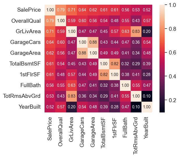
These are the variables most correlated with ‘SalePrice’
👉 ‘OverallQual’, ‘GrLivArea’ and ‘TotalBsmtSF’ are strongly correlated with ‘SalePrice’.
👉 ‘GarageCars’ and ‘GarageArea’ are also some of the most strongly correlated variables.
However, as we discussed in the last sub-point, the number of cars that fit into the garage is a consequence of the garage area.
‘GarageCars’ and ‘GarageArea’ are like twin brothers. You’ll never be able to distinguish them.
Therefore, we just need one of these variables in our analysis (we can keep ‘GarageCars’ since its correlation with ‘SalePrice’ is higher).
👉 ‘TotalBsmtSF’ and ‘1stFloor’ also seem to be twin brothers. - We can keep ‘TotalBsmtSF’ just to say that our first guess was right
👉 ‘FullBath’
👉 ‘TotRmsAbvGrd’ and ‘GrLivArea’, twin brothers again.
👉 ‘YearBuilt’… It seems that ‘YearBuilt’ is slightly correlated with ‘SalePrice’.
Let’s proceed to the scatter plots.
Scatter plots between ‘SalePrice’ and correlated variables#
#scatterplot
sns.set()
cols = ['SalePrice', 'OverallQual', 'GrLivArea', 'GarageCars', 'TotalBsmtSF', 'FullBath', 'YearBuilt']
sns.pairplot(df_train[cols], size = 2.5)
plt.show();
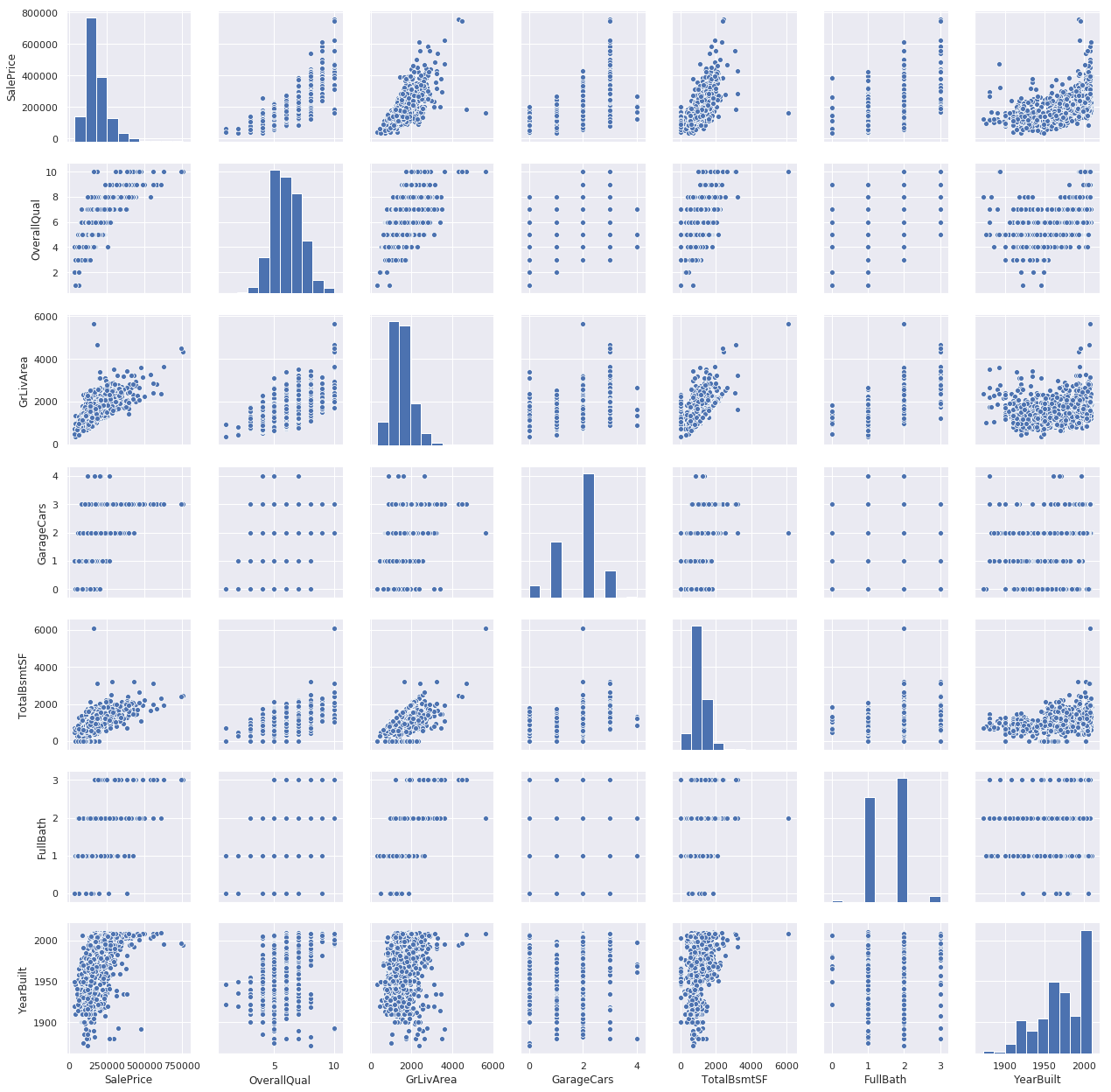
Mega scatter plot gives us a reasonable idea about variables relationships.
One of the figures we may find interesting is the one between ‘TotalBsmtSF’ and ‘GrLiveArea’.
In this figure we can see the dots drawing a linear line, which almost acts like a border. It totally makes sense that the majority of the dots stay below that line. Basement areas can be equal to the above ground living area, but it is not expected a basement area bigger than the above ground living area.
The plot concerning ‘SalePrice’ and ‘YearBuilt’ can also make us think. In the bottom of the ‘dots cloud’, we see what almost appears to be a shy exponential function (be creative). We can also see this same tendency in the upper limit of the ‘dots cloud’ (be even more creative). Also, notice how the set of dots regarding the last years tend to stay above this limit (I just wanted to say that prices are increasing faster now).
Let’s move forward to what’s missing: missing data!
Missing data#
Important questions when thinking about missing data:
How prevalent is the missing data?
Is missing data random or does it have a pattern?
The answer to these questions is important for practical reasons because missing data can imply a reduction of the sample size. This can prevent us from proceeding with the analysis. Moreover, from a substantive perspective, we need to ensure that the missing data process is not biased and hidding an inconvenient truth.
#missing data
total = df_train.isnull().sum().sort_values(ascending=False)
percent = (df_train.isnull().sum()/df_train.isnull().count()).sort_values(ascending=False)
missing_data = pd.concat([total, percent], axis=1, keys=['Total', 'Percent'])
missing_data.head(20)
| Total | Percent | |
|---|---|---|
| PoolQC | 1453 | 0.995205 |
| MiscFeature | 1406 | 0.963014 |
| Alley | 1369 | 0.937671 |
| Fence | 1179 | 0.807534 |
| MasVnrType | 872 | 0.597260 |
| FireplaceQu | 690 | 0.472603 |
| LotFrontage | 259 | 0.177397 |
| GarageYrBlt | 81 | 0.055479 |
| GarageCond | 81 | 0.055479 |
| GarageType | 81 | 0.055479 |
| GarageFinish | 81 | 0.055479 |
| GarageQual | 81 | 0.055479 |
| BsmtFinType2 | 38 | 0.026027 |
| BsmtExposure | 38 | 0.026027 |
| BsmtQual | 37 | 0.025342 |
| BsmtCond | 37 | 0.025342 |
| BsmtFinType1 | 37 | 0.025342 |
| MasVnrArea | 8 | 0.005479 |
| Electrical | 1 | 0.000685 |
| Id | 0 | 0.000000 |
Let’s analyse this to understand how to handle the missing data.
👉 We’ll consider that when more than 15% of the data is missing, we should delete the corresponding variable and pretend it never existed. This means that we will not try any trick to fill the missing data in these cases.
👉 There is a set of variables (e.g. ‘PoolQC’, ‘MiscFeature’, ‘Alley’, etc.) that we should delete. None of these variables seem to be very important, since most of them are not aspects in which we think about when buying a house (maybe that’s the reason why data is missing?).
👉 Variables like ‘PoolQC’, ‘MiscFeature’ and ‘FireplaceQu’ are strong candidates for outliers, so we’ll be happy to delete them.
👉 For other cases, we can see that ‘GarageX’ variables have the same number of missing data. I bet missing data refers to the same set of observations (although I will not check it; it’s just 5%). Since the most important information regarding garages is expressed by ‘GarageCars’ and considering that we are just talking about 5% of missing data, I’ll delete the mentioned ‘GarageX’ variables. The same logic applies to ‘BsmtX’ variables.
👉 Regarding ‘MasVnrArea’ and ‘MasVnrType’, we can consider that these variables are not essential. Furthermore, they have a strong correlation with ‘YearBuilt’ and ‘OverallQual’ which are already considered. Thus, we will not lose information if we delete ‘MasVnrArea’ and ‘MasVnrType’.
👉 Finally, we have one missing observation in ‘Electrical’. Since it is just one observation, we’ll delete this observation and keep the variable.
In summary, to handle missing data, we’ll delete all the variables with missing data, except the variable ‘Electrical’. In ‘Electrical’ we’ll just delete the observation with missing data.
#dealing with missing data
df_train = df_train.drop(columns=(missing_data[missing_data['Total'] > 1]).index)
df_train = df_train.drop(df_train.loc[df_train['Electrical'].isnull()].index)
df_train.isnull().sum().max() #just checking that there's no missing data missing...
0
Outliers#
Outliers is also something that we should be aware of. Why? Because outliers can markedly affect our models and can be a valuable source of information, providing us insights about specific behaviours.
Outliers is a complex subject and it deserves more attention. Here, we’ll just do a quick analysis through the standard deviation of ‘SalePrice’ and a set of scatter plots.
Univariate analysis#
The primary concern here is to establish a threshold that defines an observation as an outlier. To do so, we’ll standardize the data. In this context, data standardization means converting data values to have mean of 0 and a standard deviation of 1.
#standardizing data
saleprice_scaled = StandardScaler().fit_transform(df_train['SalePrice'].values.reshape(-1, 1))
low_range = saleprice_scaled[saleprice_scaled.ravel().argsort()][:10]
high_range = saleprice_scaled[saleprice_scaled.ravel().argsort()][-10:]
print('outer range (low) of the distribution:')
print(low_range)
print('\nouter range (high) of the distribution:')
print(high_range)
outer range (low) of the distribution:
[[-1.83820775]
 [-1.83303414]
 [-1.80044422]
 [-1.78282123]
 [-1.77400974]
 [-1.62295562]
 [-1.6166617 ]
 [-1.58519209]
 [-1.58519209]
 [-1.57269236]]

outer range (high) of the distribution:
[[3.82758058]
 [4.0395221 ]
 [4.49473628]
 [4.70872962]
 [4.728631  ]
 [5.06034585]
 [5.42191907]
 [5.58987866]
 [7.10041987]
 [7.22629831]]
How ‘SalePrice’ looks with her new clothes:
Low range values are similar and not too far from 0.
High range values are far from 0 and the 7.something values are really out of range.
For now, we’ll not consider any of these values as an outlier but we should be careful with those two 7.something values.
Bivariate analysis#
We already know the following scatter plots by heart. However, when we look to things from a new perspective, there’s always something to discover.
#bivariate analysis saleprice/grlivarea
var = 'GrLivArea'
data = pd.concat([df_train['SalePrice'], df_train[var]], axis=1)
data.plot.scatter(x=var, y='SalePrice', ylim=(0,800000));
What has been revealed:
👉 The two values with bigger ‘GrLivArea’ seem strange and they are not following the crowd. We can speculate why this is happening. These two points are not representative of the typical case. Therefore, we’ll define them as outliers and delete them.
👉 The two observations in the top of the plot are those 7.something observations that we said we should be careful about. They look like two special cases, however they seem to be following the trend. For that reason, we will keep them.
#deleting points
df_train.sort_values(by = 'GrLivArea', ascending = False)[:2]
df_train = df_train.drop(df_train[df_train['Id'] == 1299].index)
df_train = df_train.drop(df_train[df_train['Id'] == 524].index)
#bivariate analysis saleprice/grlivarea
var = 'TotalBsmtSF'
data = pd.concat([df_train['SalePrice'], df_train[var]], axis=1)
data.plot.scatter(x=var, y='SalePrice', ylim=(0,800000));
We can feel tempted to eliminate some observations (e.g. TotalBsmtSF > 3000) but I suppose it’s not worth it. We can live with that, so we’ll not do anything.
Testing assumptions#
Let’s do testing for the assumptions underlying the statistical bases for multivariate analysis. We already did some data cleaning and discovered a lot about ‘SalePrice’. Now it’s time to go deep and understand how ‘SalePrice’ complies with the statistical assumptions that enables us to apply multivariate techniques.
According to Hair et al. (2013), four assumptions should be tested:
Normality - When we talk about normality what we mean is that the data should look like a normal distribution. This is important because several statistic tests rely on this (e.g. t-statistics). In this exercise we’ll just check univariate normality for ‘SalePrice’ (which is a limited approach). Remember that univariate normality doesn’t ensure multivariate normality (which is what we would like to have), but it helps. Another detail to take into account is that in big samples (>200 observations) normality is not such an issue. However, if we solve normality, we avoid a lot of other problems (e.g. heteroscedacity) so that’s the main reason why we are doing this analysis.
Homoscedasticity - Homoscedasticity refers to the ‘assumption that dependent variable(s) exhibit equal levels of variance across the range of predictor variable(s)’ (Hair et al., 2013). Homoscedasticity is desirable because we want the error term to be the same across all values of the independent variables.
Linearity- The most common way to assess linearity is to examine scatter plots and search for linear patterns. If patterns are not linear, it would be worthwhile to explore data transformations. However, we’ll not get into this because most of the scatter plots we’ve seen appear to have linear relationships.
Absence of correlated errors - Correlated errors, like the definition suggests, happen when one error is correlated to another. For instance, if one positive error makes a negative error systematically, it means that there’s a relationship between these variables. This occurs often in time series, where some patterns are time related. We’ll also not get into this. However, if you detect something, try to add a variable that can explain the effect you’re getting. That’s the most common solution for correlated errors.
Normality#
The point here is to test ‘SalePrice’ in a very lean way. We’ll do this paying attention to:
Histogram - Kurtosis and skewness.
Normal probability plot - Data distribution should closely follow the diagonal that represents the normal distribution.
#histogram and normal probability plot
sns.distplot(df_train['SalePrice'], fit=norm);
fig = plt.figure()
res = stats.probplot(df_train['SalePrice'], plot=plt)
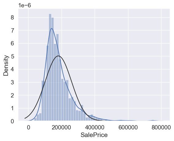
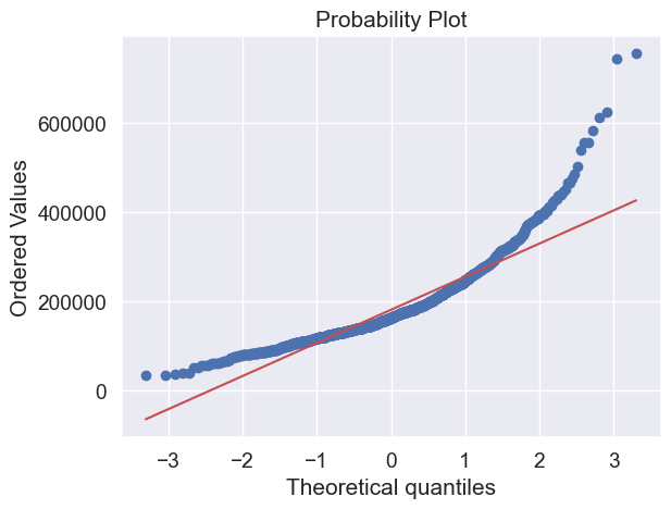
Ok, ‘SalePrice’ is not normal. It shows ‘peakedness’, positive skewness and does not follow the diagonal line.
But everything’s not lost. A simple data transformation can solve the problem.
In case of positive skewness, log transformations usually works well.
#applying log transformation
df_train['SalePrice'] = np.log(df_train['SalePrice'])
#transformed histogram and normal probability plot
sns.distplot(df_train['SalePrice'], fit=norm);
fig = plt.figure()
res = stats.probplot(df_train['SalePrice'], plot=plt)
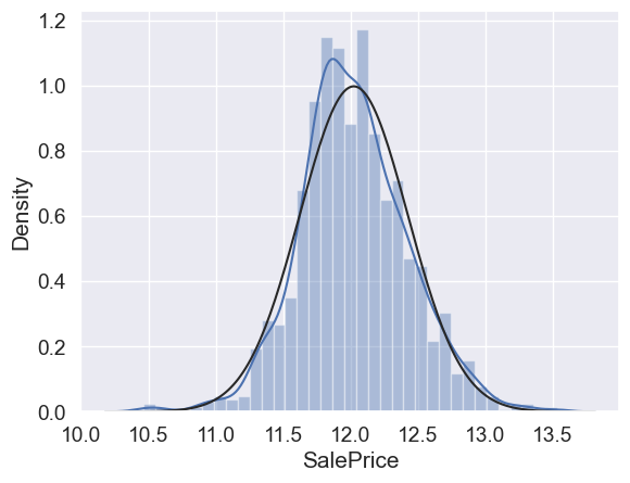
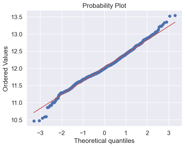
Done! Let’s check what’s going on with ‘GrLivArea’.
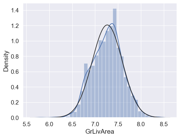
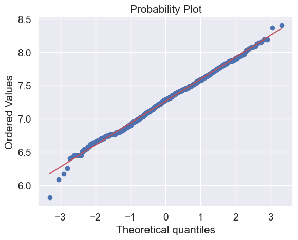
#histogram and normal probability plot
sns.distplot(df_train['GrLivArea'], fit=norm);
fig = plt.figure()
res = stats.probplot(df_train['GrLivArea'], plot=plt)
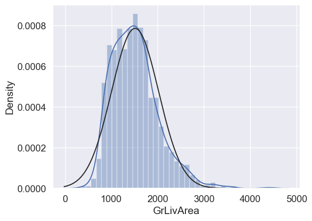
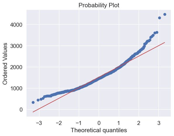
Skewness
#data transformation
df_train['GrLivArea'] = np.log(df_train['GrLivArea'])
#transformed histogram and normal probability plot
sns.distplot(df_train['GrLivArea'], fit=norm);
fig = plt.figure()
res = stats.probplot(df_train['GrLivArea'], plot=plt)
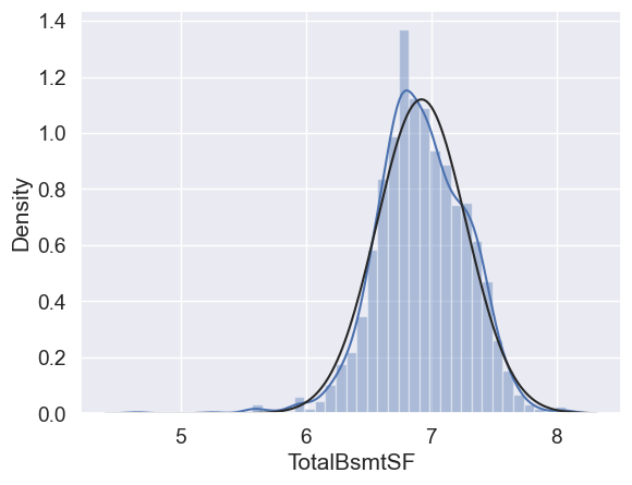
#histogram and normal probability plot
sns.distplot(df_train['TotalBsmtSF'], fit=norm);
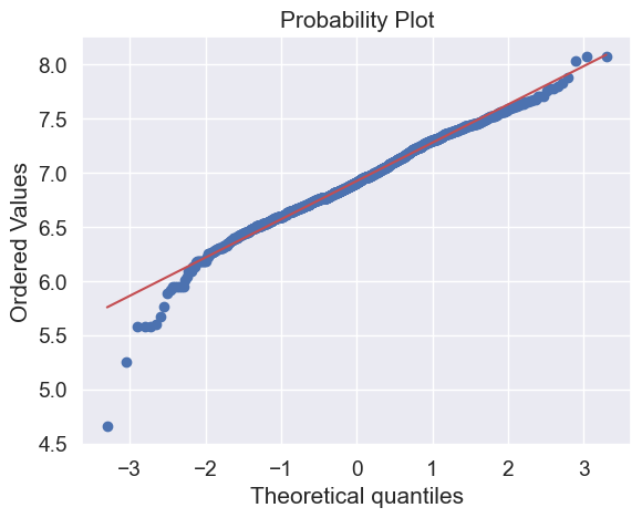
fig = plt.figure()
res = stats.probplot(df_train['TotalBsmtSF'], plot=plt)
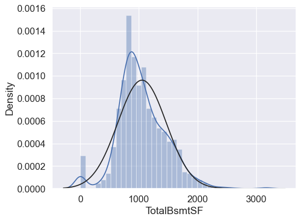
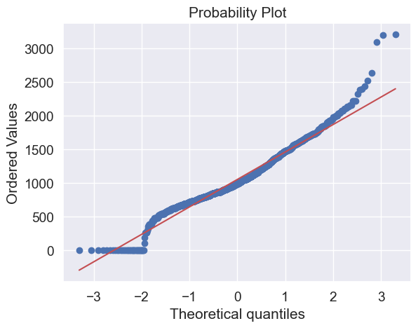
What do we have here?
Something that, in general, presents skewness.
A significant number of observations with value zero (houses without basement).
A big problem because the value zero doesn’t allow us to do log transformations.
👉 To apply a log transformation here, we’ll create a variable that can get the effect of having or not having basement (binary variable).
👉 Then, we’ll do a log transformation to all the non-zero observations, ignoring those with value zero. This way we can transform data, without losing the effect of having or not basement.
#create column for new variable (one is enough because it's a binary categorical feature)
#if area>0 it gets 1, for area==0 it gets 0
df_train['HasBsmt'] = pd.Series(len(df_train['TotalBsmtSF']), index=df_train.index)
df_train['HasBsmt'] = 0
df_train.loc[df_train['TotalBsmtSF']>0,'HasBsmt'] = 1
#transform data
df_train.loc[df_train['HasBsmt']==1,'TotalBsmtSF'] = np.log(df_train['TotalBsmtSF'])
#histogram and normal probability plot
sns.distplot(df_train[df_train['TotalBsmtSF']>0]['TotalBsmtSF'], fit=norm);
fig = plt.figure()
res = stats.probplot(df_train[df_train['TotalBsmtSF']>0]['TotalBsmtSF'], plot=plt)
Homoscedasticity#
The best approach to test homoscedasticity for two metric variables is graphically. Departures from an equal dispersion are shown by such shapes as cones (small dispersion at one side of the graph, large dispersion at the opposite side) or diamonds (a large number of points at the center of the distribution).
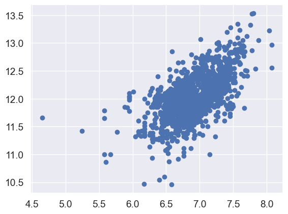
Starting by ‘SalePrice’ and ‘GrLivArea’…
#scatter plot
plt.scatter(df_train['GrLivArea'], df_train['SalePrice']);
Older versions of this scatter plot (previous to log transformations), had a conic shape (go back and check ‘Scatter plots between ‘SalePrice’ and correlated variables (move like Jagger style)’). As you can see, the current scatter plot doesn’t have a conic shape anymore. That’s the power of normality! Just by ensuring normality in some variables, we solved the homoscedasticity problem.
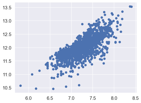
Now let’s check ‘SalePrice’ with ‘TotalBsmtSF’.
#scatter plot
plt.scatter(df_train[df_train['TotalBsmtSF']>0]['TotalBsmtSF'], df_train[df_train['TotalBsmtSF']>0]['SalePrice']);
We can say that, in general, ‘SalePrice’ exhibit equal levels of variance across the range of ‘TotalBsmtSF’. Cool!
Dummy variables#
Easy mode.
#convert categorical variable into dummy
df_train = pd.get_dummies(df_train)
Conclusion#
👉 We applied strategies from Hair et al. (2013), including:
Analyzing ‘SalePrice’ alone and with correlated variables
Handling missing data and outliers
Testing statistical assumptions
Transforming categorical variables to dummies
👉 Next steps:
Predict ‘SalePrice’ behavior
Consider different approaches:
Regularized linear regression
Ensemble methods
Other techniques
The choice of method is up to you to explore and determine