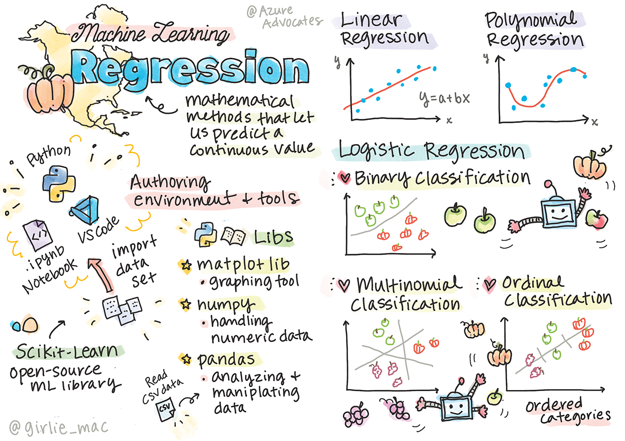
Regression#
Regression is a type of machine learning algorithm used to predict a continuous output variable based on one or more input variables. It is a fundamental technique in statistics and data analysis, and it is widely used in various fields such as finance, economics, and science.
The goal of regression analysis is to establish a relationship between the input variables (also known as independent variables) and the output variable (also known as the dependent variable). This relationship is typically represented by a mathematical equation that can be used to make predictions about the output variable for new input values.
There are several types of regression algorithms, including:
Simple Linear Regression: This is the simplest form of regression, involving a single input variable and a single output variable. The relationship between the variables is assumed to be linear, meaning that the output variable changes in a constant amount for each unit change in the input variable.
Multiple Linear Regression: This type of regression involves multiple input variables and a single output variable. The relationship between the variables is assumed to be linear, meaning that the output variable changes in a constant amount for each unit change in the input variables.
Polynomial Regression: This type of regression involves a single input variable and a single output variable, but the relationship between the variables is assumed to be non-linear. The relationship is represented by a polynomial equation, which can be used to make predictions about the output variable for new input values.
There are more types of regression algorithms, which we will explore in the upcoming lessons.
Linear Regression in one variable#
Linear regression will find a straight line that will try to best fit the data provided. It does so by learning the slope of the line, and the bais term (y-intercept)
Given a table:
size of house(int sq. ft) (x) |
price in $1000(y) |
|---|---|
450 |
100 |
324 |
78 |
844 |
123 |
Our hypothesis (prediction) is: $\(h_\theta(x) = \theta_0 + \theta_1x\)$ Will give us an equation of line that will predict the price.
The above equation is nothing but the equation of line.
When we say the machine learns, we are actually adjusting the parameters \(\theta_0\) and \(\theta_1\).
So for a new x (size of house) we will insert the value of x in the above equation and produce a value \(\hat y\) (our prediction)
Our prediction \(\hat y\) will not always be accurate, and will have a certain error which we will define by an equation.
We will also need this equation to minimise the error, this equation is called as loss function.
One of the most used one is called Mean Squared Error (MSE) which is nothing but the means of all the errors squared.
Where,
\(m\) = the number of training examples
\(x_i\) = the value of x at ith row
\(y_i\) = the actual value at the ith row
\(h_\theta(x)\) = our prediction function that predicts \(\hat y\)
Why square the difference?
The error will be positive
If you take the absolute function (to cover point 1), the absolute function isn’t differentiable at the origin. Hence, we square the error.
Why \(\frac{1}{2m}\) instead of \(\frac{1}{m}\) ?
As we will see later, when we differentiate the squared error, the \(\frac{1}{2}\) will cancel out. If we don’t do that we’ll be stuck with a \(2\) in the equation which is useless.
Minimising the cost function#
Our objective function is
$\(\displaystyle \operatorname*{argmin}_\theta J(\theta)\)$#
Which simply means, find the value of \(\theta\) that minimises the error function \(J(\theta)\).
In order to do that, we will differentiate our cost function.
When we differentiate it, it will give us gradient, which is the direction in which the error will be reduced.
Upon having the gradient, we will simply update our \(\theta\) values to reflect that step (a step in the direction of lower error)
So, the update rule is the following equation
Where,
\(\alpha\) = learning rate. Which is the rate at which we will travel to the direction of the lower error.
This process is nothing but Gradient Descent. There are few version of gradient descent, few of them are:
Batch Gradient Descent: Go through all your input samples, compute the gradient once, and then update \(\theta\) s.
Stochastic Gradient Descent: Go through a single sample, compute gradient, update \(\theta\) s, repeat \(m\) times
Mini Batch Gradient Descent: Go through a batch of \(k\) samples, compute gradient, update \(\theta\) s, repeat \(\frac{m}{k}\) times.
Differentiating the loss function:#
In the update rule:
The important part is calculating the derivative. Since we have two variables, we will have two derivatives, one for \(\theta_0\) and another for \(\theta_1\).
So the first equation is:
$
$
Similarly, for \(\theta_1\)
$
$
We will implement Batch Gradient Descent i.e. we’ll update the gradients after 1 pass through the entire dataset. Our Algorithm hence becomes:
Repeat till convergence:
\(\theta_0= \theta_0 - \frac{1}{m}\sum_{i=0}^m{(h_\theta(x_i) - y_i)} \)
\(\theta_1= \theta_1 - \frac{1}{m}\sum_{i=0}^m{(h_\theta(x_i) - y_i)}(x) \)
Implementation#
from __future__ import division, print_function
import numpy as np
import pandas as pd
import matplotlib.pyplot as plt

# Creates a table data structure which is easy to manipulate
df = pd.read_csv("machine_learning_andrewng/ex1data1.csv", header=None)
df.rename(columns={0: 'population', 1: 'profit'}, inplace=True)
df.head()
| population | profit | |
|---|---|---|
| 0 | 6.1101 | 17.5920 |
| 1 | 5.5277 | 9.1302 |
| 2 | 8.5186 | 13.6620 |
| 3 | 7.0032 | 11.8540 |
| 4 | 5.8598 | 6.8233 |
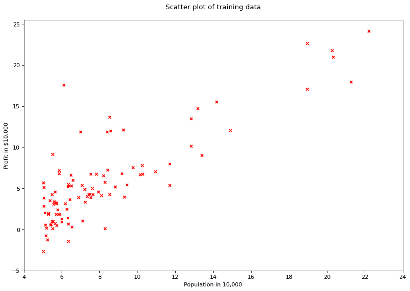
# visualising the data
fig = plt.figure(num=None, figsize=(12, 8), dpi=80, facecolor='w')
plt.scatter(df['population'], df['profit'], marker='x', color='red', s=20)
plt.xlim([4, 24])
plt.xticks(range(4, 26, 2))
plt.yticks(range(-5, 30, 5))
plt.xlabel("Population in 10,000")
plt.ylabel("Profit in $10,000")
plt.title("Scatter plot of training data\n")
plt.show()
class LinearRegression(object):
    """Performs Linear Regression using Batch Gradient
    Descent."""
    def __init__(self, X, y, alpha=0.01, n_iterations=5000):
        """Initialise variables.

        Parameters
        ----------
        y : numpy array like, output / dependent variable
        X : numpy array like, input / independent variables
        alpha : float, int. Learning Rate
        n_iterations : Number of maximum iterations to perform
            gradient descent
        """
        self.y = y
        self.X = self._hstack_one(X)
        self.thetas = np.zeros((self.X.shape[1], 1))
        self.n_rows = self.X.shape[0]
        self.alpha = alpha
        self.n_iterations = n_iterations
        print("Cost before fitting: {0:.2f}".format(self.cost()))

    @staticmethod
    def _hstack_one(input_matrix):
        """Horizontally stack a column of ones for the coefficients
        of the bias terms

        Parameters
        ----------
        input_matrix: numpy array like (N x M). Where N = number of
            examples. M = Number of features.

        Returns
        -------
        numpy array with stacked column of ones (N x M + 1)
        """
        return np.hstack((np.ones((input_matrix.shape[0], 1)),
                              input_matrix))

    def cost(self, ):
        """Calculates the cost of current configuration"""
        return (1 / (2 * self.n_rows)) * np.sum(
            (self.X.dot(self.thetas) - self.y) ** 2)

    def predict(self, new_X):
        """Predict values using current configuration

        Parameters
        ----------
        new_X : numpy array like
        """

        new_X = self._hstack_one(new_X)
        return new_X.dot(self.thetas)

    def batch_gradient(self, ):
        h = self.X.dot(self.thetas) - self.y
        h = np.multiply(self.X, h)
        h = np.sum(h, axis=0)
        return h.reshape(-1, 1)

    def batch_gradient_descent(self, ):
        alpha_by_m = self.alpha / self.n_rows
        for i in range(self.n_iterations):
            self.thetas = self.thetas - (alpha_by_m * self.batch_gradient())
            cost = self.cost()
            print("Iteration: {0} Loss: {1:.5f}\r".format(i + 1, cost), end="")
X = df['population'].values.reshape(-1, 1)
y = df['profit'].values.reshape(-1, 1)
lr = LinearRegression(X, y)
lr.batch_gradient_descent()
Cost before fitting: 32.07
Iteration: 5000 Loss: 4.47697
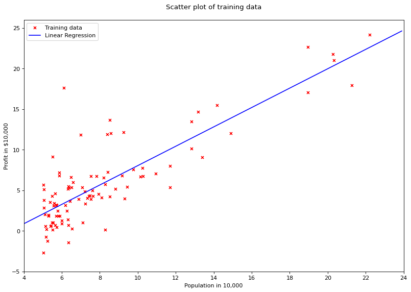
# plot regression line
X = np.arange(4, 24, 0.1).reshape(-1, 1)
fig = plt.figure(num=None, figsize=(12, 8), dpi=80, facecolor='w')
plt.scatter(df['population'], df['profit'], marker='x', color='red', s=20, label='Training data')
plt.plot(X, lr.predict(X), color='blue', label='Linear Regression')
plt.xlim([4, 24])
plt.xticks(range(4, 26, 2))
plt.yticks(range(-5, 30, 5))
plt.xlabel("Population in 10,000")
plt.ylabel("Profit in $10,000")
plt.title("Scatter plot of training data\n")
plt.legend()
plt.show()
def cost(theta_0, theta_1):
    """Calculate the cost with given weights

    Parameters
    ----------
    theta_0 : numpy array like, weights dim 0
    theta_1 : numpy array like, weights dim 1

    Returns
    -------
    float, cost
    """

    X = df['population'].values
    y = df['profit'].values
    X = X.reshape(-1, 1)
    y = y.reshape(-1, 1)
    X = np.hstack((np.ones((X.shape[0], 1)), X))
    n_rows = X.shape[0]
    thetas = np.array([theta_0, theta_1]).reshape(-1, 1)
    return (1/(2*n_rows)) * sum((X.dot(thetas) - y)**2)[0]

def prepare_cost_matrix(theta0_matrix, theta1_matrix):
    """Prepares cost matrix for various weights to
    create a 3D representation of cost. Every value
    in the cost matrix represents the cost for theta
    values in the theta matrices.

    Parameters
    ----------
    theta0_matrix : numpy array like, weights dim 0
    theta1_matrix : numpy array like, weights dim 1
    """
    J_matrix = np.zeros(theta0_matrix.shape)
    row, col = theta0_matrix.shape
    for x in range(row):
        for y in range(col):
            J_matrix[x][y] = cost(theta0_matrix[x][y], theta1_matrix[x][y])
    return J_matrix

theta_0 = np.arange(-5, 1, 0.01)
theta_1 = np.arange(0.6, 1.2, 0.001)
theta_0, theta_1 = np.meshgrid(theta_0, theta_1)
J_matrix = prepare_cost_matrix(theta_1, theta_0)
from mpl_toolkits.mplot3d import Axes3D
from matplotlib import cm
from matplotlib.ticker import LinearLocator, FormatStrFormatter
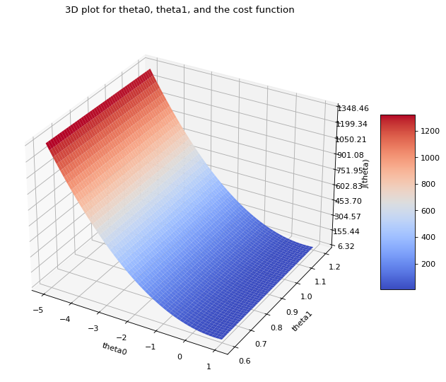
fig = plt.figure(num=None, figsize=(12, 8), dpi=80, facecolor='w')
ax = fig.add_subplot(111, projection='3d')
surf = ax.plot_surface(theta_0, theta_1, J_matrix, cmap=cm.coolwarm)
ax.zaxis.set_major_locator(LinearLocator(10))
ax.set_xlabel("theta0")
ax.set_ylabel("theta1")
ax.set_zlabel("J(theta)")
ax.zaxis.set_major_formatter(FormatStrFormatter('%.02f'))
fig.colorbar(surf, shrink=0.5, aspect=5)
plt.title("3D plot for theta0, theta1, and the cost function\n")
plt.show()
Multivariable regression#
The update rule stated above can be extended to as many \(\theta\) s as possible using matrix notation. the key is to store the \(\theta\) s in one vector and the input data in a matrix then take a dot product of them.
Implementation#
df = pd.read_csv("machine_learning_andrewng/ex1data2.csv", header=None)
df.head()
| 0 | 1 | 2 | |
|---|---|---|---|
| 0 | 2104 | 3 | 399900 |
| 1 | 1600 | 3 | 329900 |
| 2 | 2400 | 3 | 369000 |
| 3 | 1416 | 2 | 232000 |
| 4 | 3000 | 4 | 539900 |
X = df.iloc[:, [0, 1]].values
y = df.iloc[:, [2]].values
from sklearn.preprocessing import StandardScaler

scaler_X = StandardScaler()
scaler_Y = StandardScaler()
X = scaler_X.fit_transform(X)
y = scaler_Y.fit_transform(y)
lr = LinearRegression(X, y, alpha=0.1, n_iterations=1000)
lr.batch_gradient_descent()
Cost before fitting: 0.50
Iteration: 1000 Loss: 0.13353
X_test = np.array([2104, 3]).reshape(1, 2)
print("Testing on : {0}".format(X_test[0]))
X_test = scaler_X.transform(X_test)
prediction = lr.predict(X_test)
print("Prediction(Scaled): {0:.2f}".format(prediction[0][0]))
print("Prediction(Unscaled): {0:.2f}".format(scaler_Y.inverse_transform(prediction)[0][0]))
Testing on : [2104    3]
Prediction(Scaled): 0.13
Prediction(Unscaled): 356283.11
Assumptions in Linear Regression:#
Normally distributed Residuals Residuals should be normally distributed. This can be checked using histogram of residuals
Little to no Multicollinearity Multiple regression assumes that the independent variables are not highly correlated with each other. This assumption is tested using Variance Inflation Factor (VIF) values. One way to deal with multicollinearity is subtracting mean.
Homoscedasticity This assumption states that the variance of error terms are similar across the values of the independent variables. A plot of standardized residuals versus predicted values can show whether points are equally distributed across all values of the independent variables.
Dummy variable trap#
This occurs when there is redundant information due to OneHotEncoder. Eg if there are two cities, New York and California, then a since City_New_York with value 0 or 1 is enough to preserve the information. If you make two columns City_New_York and City_California then both will portray same information, just opposite values. This introduces multicollinearity. When there are many unrelated featueres, the model can learn a lot from those. But when there are less features, then the model will be unstable and will undergo huge changes with little change in input value.
Dummy variable trap can be avoided by dropping one feature off every subset of dummy variables.
import numpy as np
import pandas as pd

from sklearn.datasets import make_regression
from sklearn.linear_model import LinearRegression
from sklearn.model_selection import cross_val_score

# Create made up regression dataset
X, y = make_regression(n_samples=100, n_features=20, noise=0.95)
# Create a table to view it
df = pd.DataFrame(X)
df.head()
| 0 | 1 | 2 | 3 | 4 | 5 | 6 | 7 | 8 | 9 | 10 | 11 | 12 | 13 | 14 | 15 | 16 | 17 | 18 | 19 | |
|---|---|---|---|---|---|---|---|---|---|---|---|---|---|---|---|---|---|---|---|---|
| 0 | 0.074232 | 1.986427 | 0.310052 | -1.004567 | 0.141186 | 1.145350 | 1.400318 | -0.881926 | -0.843096 | -1.560638 | -0.566479 | 0.351185 | 0.405732 | 0.333857 | -0.407014 | 0.923185 | 0.374436 | -1.983881 | 0.661644 | 0.513339 |
| 1 | -2.826229 | 0.627472 | -1.791484 | -0.006147 | -1.067629 | -0.323952 | -1.857131 | -0.084058 | 1.319829 | -0.285186 | -1.259155 | -0.312493 | -0.063735 | -1.125292 | -0.465324 | 0.569733 | 0.679675 | -0.304674 | 1.214460 | 0.319342 |
| 2 | 0.572795 | -0.370965 | -0.609491 | -3.127797 | -0.808524 | -2.604676 | -1.058772 | -0.980460 | -1.347285 | -0.886258 | -2.736957 | 0.820368 | 2.309269 | 1.769153 | -1.111227 | -0.829549 | 0.584717 | 0.291793 | -0.977619 | -1.043986 |
| 3 | -1.581389 | 1.714122 | 0.600613 | 0.223763 | 0.567996 | -2.146892 | 0.023523 | 1.230237 | 0.521923 | 1.476945 | 1.032412 | -1.282115 | -0.513629 | 1.197274 | 0.867149 | -1.793386 | 0.876216 | -1.515119 | -1.532318 | -0.374120 |
| 4 | -0.846028 | -0.157537 | 2.246263 | 1.230532 | -1.061811 | 0.806593 | -0.960286 | -2.075879 | 0.016584 | 0.503500 | 0.137756 | 0.172076 | -0.989669 | -0.549751 | 1.766336 | 0.973990 | -1.347037 | -1.438085 | -1.793198 | -0.386394 |
Results on a dataset with no multicollinearity#
# Cross Validation will fit the classifier N number of times
# and display the accuracies
cv = cross_val_score(LinearRegression(), X, y, cv=10)
print("Mean: {}".format(cv.mean()))
print("Values: {}".format(cv))
Mean: 0.999944526095
Values: [ 0.99996679  0.99996035  0.99985266  0.99996614  0.99995686  0.99994011
  0.99992176  0.99997001  0.99994873  0.99996186]
# Create the dataset once again. This time, introduce high
# multicollinearity by setting low rank to the input matrix
X, y = make_regression(n_samples=100, n_features=20, noise=0.95, effective_rank=1)
df = pd.DataFrame(X)
df.head()
| 0 | 1 | 2 | 3 | 4 | 5 | 6 | 7 | 8 | 9 | 10 | 11 | 12 | 13 | 14 | 15 | 16 | 17 | 18 | 19 | |
|---|---|---|---|---|---|---|---|---|---|---|---|---|---|---|---|---|---|---|---|---|
| 0 | 0.015846 | -0.010931 | -0.004674 | 0.003822 | -0.023871 | -0.017512 | 0.044750 | 0.009582 | -0.015291 | -0.016862 | 0.027048 | 0.004653 | 0.012857 | 0.015904 | -0.026063 | -0.006431 | 0.029526 | 0.012398 | 0.005457 | 0.012917 |
| 1 | 0.020191 | 0.014001 | 0.006417 | -0.003025 | -0.011963 | -0.007565 | 0.013667 | -0.008957 | 0.036918 | -0.028306 | -0.010519 | -0.031603 | 0.030384 | -0.000335 | 0.000405 | -0.029291 | 0.005563 | -0.035104 | 0.023762 | -0.001103 |
| 2 | -0.009227 | -0.013174 | -0.080700 | 0.021887 | -0.041854 | 0.052632 | 0.000175 | 0.017286 | -0.021256 | 0.011598 | -0.019671 | -0.003535 | 0.047776 | -0.023163 | -0.007540 | 0.013366 | -0.036634 | -0.032115 | -0.054735 | 0.030348 |
| 3 | -0.033374 | 0.002136 | 0.009405 | 0.020186 | -0.002358 | -0.007324 | -0.030595 | 0.013745 | 0.012005 | 0.001523 | 0.009838 | 0.012011 | -0.009667 | -0.000170 | 0.025990 | 0.012361 | 0.002625 | -0.001620 | 0.021952 | -0.003477 |
| 4 | -0.005361 | 0.027710 | 0.027310 | 0.002298 | 0.014358 | -0.010233 | -0.031642 | 0.000922 | -0.008463 | -0.019281 | 0.018650 | 0.004970 | 0.060408 | 0.011731 | -0.014682 | -0.055579 | -0.011830 | 0.019722 | 0.003625 | 0.003970 |
Results on dataset with high multicollinearity#
# Cross Validation will fit the classifier N number of times
# and display the accuracies
cv = cross_val_score(LinearRegression(), X, y, cv=10)
print("Mean: {}".format(cv.mean()))
print("Values: {}".format(cv))
Mean: 0.927965134304
Values: [ 0.8348102   0.95336766  0.93501047  0.95455964  0.8854501   0.95326037
  0.9354691   0.92986913  0.95585656  0.94199813]
Why is Polynomial Linear Regression “Linear” ?#
The answer lies the equation on how polynomial linear regression is implemented.
The outcome y is defined as the linear combination of the independent variables.
That’s the reason it is linear. The outcome has nothing to do with the non-linearities in the independent variables
import pandas as pd
import matplotlib.pyplot as plt
import numpy as np

df = pd.read_csv('Position_Salaries.csv')
X = df.iloc[:, 1:2]   # Using 1:2 as indices will give us np array of dim (10, 1)
y = df.iloc[:, 2]

df.head()
| Position | Level | Salary | |
|---|---|---|---|
| 0 | Business Analyst | 1 | 45000 |
| 1 | Junior Consultant | 2 | 50000 |
| 2 | Senior Consultant | 3 | 60000 |
| 3 | Manager | 4 | 80000 |
| 4 | Country Manager | 5 | 110000 |
from sklearn.linear_model import LinearRegression
lin_reg = LinearRegression()
lin_reg.fit(X, y)
LinearRegression()In a Jupyter environment, please rerun this cell to show the HTML representation or trust the notebook.
On GitHub, the HTML representation is unable to render, please try loading this page with nbviewer.org.
LinearRegression()
Add Polynomial features using PolynomialFeatures class from sklearn.preprocessing
from sklearn.preprocessing import PolynomialFeatures
poly_reg_2 = PolynomialFeatures(degree=2)
poly_reg_3 = PolynomialFeatures(degree=3)
X_poly_2 = poly_reg_2.fit_transform(X)
X_poly_3 = poly_reg_3.fit_transform(X)
X_poly_2
array([[  1.,   1.,   1.],
       [  1.,   2.,   4.],
       [  1.,   3.,   9.],
       [  1.,   4.,  16.],
       [  1.,   5.,  25.],
       [  1.,   6.,  36.],
       [  1.,   7.,  49.],
       [  1.,   8.,  64.],
       [  1.,   9.,  81.],
       [  1.,  10., 100.]])
Notice that the first column containing 1 is already added automatically
Now we can make LinearRegression object using these newly added polynomial features
lin_reg_poly_2 = LinearRegression().fit(X_poly_2, y)
lin_reg_poly_3 = LinearRegression().fit(X_poly_3, y)
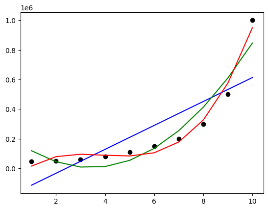
plt.scatter(X, y, color='black')
plt.plot(X, lin_reg.predict(X), color='b')
plt.plot(X, lin_reg_poly_2.predict(poly_reg_2.fit_transform(X)), color='g')
plt.plot(X, lin_reg_poly_3.predict(poly_reg_3.fit_transform(X)), color='r')
plt.show()
Support Vector Regression#
SVR is a type of Support Vector Machine (SVM) used for regression problems. It is a non-linear model that uses a kernel function to map the input data into a higher-dimensional space where a linear model can be used. The model aims to find a hyperplane that best fits the data points in this higher-dimensional space, allowing for non-linear relationships to be modeled.
SVR is particularly useful when dealing with complex datasets that exhibit non-linear patterns. By using a kernel function, SVR can effectively handle non-linear relationships between variables, making it a powerful tool for regression analysis.
Key Concepts in SVR:#
Kernel Function: SVR uses a kernel function to map the input data into a higher-dimensional space. This allows for non-linear relationships to be modeled. Common kernel functions include the radial basis function (RBF), polynomial, and sigmoid kernels.
Regularization Parameter ©: This parameter controls the trade-off between achieving a low error on the training data and ensuring the model is not too complex. A smaller C value leads to a wider margin, allowing more data points to be within the margin, potentially increasing the model’s bias but reducing variance. Conversely, a larger C value leads to a narrower margin, reducing the model’s bias but increasing its variance.
Epsilon (ε): This parameter determines the width of the ε-insensitive zone around the regression line. Data points within this zone are considered to have zero error, while points outside this zone contribute to the error. The choice of ε depends on the scale of the target variable and the desired level of robustness to outliers.
Kernel Parameters: The choice of kernel function and its parameters (e.g., degree for polynomial kernels) can significantly impact the model’s performance. Common kernels include:
Radial Basis Function (RBF):
Kernel function: ( K(x, x’) = \exp\left(-\gamma |x - x’|^2\right) )
Parameters: γ (gamma) controls the influence of individual training samples.
Regularization Path: SVR provides a regularization path, which shows how the model’s complexity changes as the regularization parameter C is varied. This helps in selecting an appropriate value of C for the given dataset.
Implementation#
Let’s revisit the previous example of predicting the salary based on position level using SVR.
import pandas as pd
import matplotlib.pyplot as plt
import numpy as np

df = pd.read_csv('Position_Salaries.csv')
X = df.iloc[:, 1:2]   # Using 1:2 as indices will give us np array of dim (10, 1)
y = df.iloc[:, 2]

df.head()
| Position | Level | Salary | |
|---|---|---|---|
| 0 | Business Analyst | 1 | 45000 |
| 1 | Junior Consultant | 2 | 50000 |
| 2 | Senior Consultant | 3 | 60000 |
| 3 | Manager | 4 | 80000 |
| 4 | Country Manager | 5 | 110000 |
from sklearn.svm import SVR
regressor = SVR(kernel='rbf').fit(X, y)
plt.scatter(X, y)
plt.plot(X, regressor.predict(X), color='r')
plt.show()
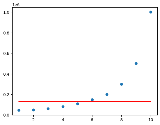
The model is very bad because we did not scale the input. Most of the models like LinearRegression automatically scale the data, but perhaps the SVR model is not widely used, it doesn’t scale the data by itself. Hence we have to manually scale the data
from sklearn.preprocessing import StandardScaler
import numpy as np

sc_X = StandardScaler()
sc_y = StandardScaler()

# Ensure X is 2D
X = np.array(X).reshape(-1, 1) if X.ndim == 1 else np.array(X)
X = sc_X.fit_transform(X)

# Reshape y to 2D
y = np.array(y).reshape(-1, 1)
y = sc_y.fit_transform(y)

# If you prefer y as a 1D array after scaling, you can flatten it
y = y.flatten()
regressor = SVR(kernel='rbf').fit(X, y)
plt.scatter(X, y)
plt.plot(X, regressor.predict(X), color='r')
plt.show()
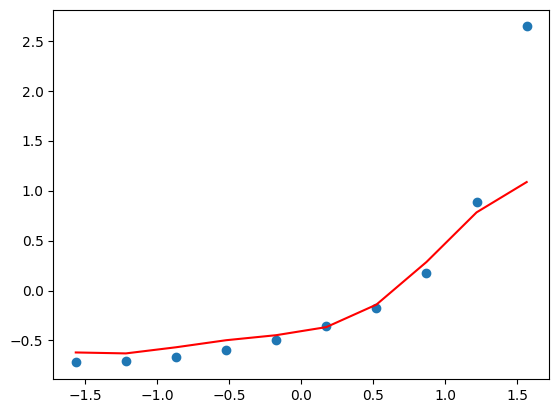
The prediction of the last point is a bit off because it is treated as an outlier by the default parameters set by SVR.
Now in order to predict a particular input, we first scale it, predict it, and inverse scale it to obtain the actual value
# Predict
X_test = np.array([[6.5]])
X_test_scaled = sc_X.transform(X_test)
y_pred_scaled = regressor.predict(X_test_scaled)

# Reshape y_pred_scaled to 2D array
y_pred_scaled = y_pred_scaled.reshape(-1, 1)

# Inverse transform
y_pred = sc_y.inverse_transform(y_pred_scaled)

print("Prediction:", y_pred[0][0])
Prediction: 252789.13921623852
y_pred
array([[252789.13921624]])
Decision Tree Regression#
Decision tree regression is a type of regression analysis that uses a decision tree model to predict a continuous outcome variable. It is a non-parametric method, meaning it does not make any assumptions about the functional form of the relationship between the independent variables and the dependent variable. Instead, it builds a tree-like structure that recursively partitions the feature space into regions, assigning a constant value to each region based on the mean of the target variable.
Key Concepts in Decision Tree Regression:#
Recursive Partitioning: The feature space is recursively partitioned into regions based on the values of the independent variables. Each partition is represented by a node in the tree, with the final partition being a leaf node containing the predicted value.
Splitting Criteria: The splitting criteria determine how the feature space is partitioned. Common criteria include mean squared error for regression tasks.
Overfitting: Decision trees can easily overfit the training data, especially if the tree is deep. Techniques like pruning can be used to prevent overfitting.
Feature Importance: Decision trees provide a measure of feature importance, which helps in understanding which features are most influential in predicting the target variable.
Regularization: Decision trees can be regularized using techniques like pruning to prevent overfitting.
Implementation#
import pandas as pd
import matplotlib.pyplot as plt
import numpy as np

df = pd.read_csv('Position_Salaries.csv')
X = df.iloc[:, 1:2]   # Using 1:2 as indices will give us np array of dim (10, 1)
y = df.iloc[:, 2]

df.head()
| Position | Level | Salary | |
|---|---|---|---|
| 0 | Business Analyst | 1 | 45000 |
| 1 | Junior Consultant | 2 | 50000 |
| 2 | Senior Consultant | 3 | 60000 |
| 3 | Manager | 4 | 80000 |
| 4 | Country Manager | 5 | 110000 |
from sklearn.tree import DecisionTreeRegressor
regressor = DecisionTreeRegressor(random_state=0).fit(X, y)
plt.scatter(X, y)
X_grid = np.arange(min(X.values), max(X.values), 0.1).reshape(-1, 1)
plt.plot(X_grid, regressor.predict(X_grid), color='r')
plt.show()
/var/folders/7m/04ssj6n96q984_6wsnr60dg00000gn/T/ipykernel_92876/3445426962.py:2: DeprecationWarning: Conversion of an array with ndim > 0 to a scalar is deprecated, and will error in future. Ensure you extract a single element from your array before performing this operation. (Deprecated NumPy 1.25.)
  X_grid = np.arange(min(X.values), max(X.values), 0.1).reshape(-1, 1)
/opt/homebrew/Caskroom/miniconda/base/envs/ml-notes/lib/python3.12/site-packages/sklearn/base.py:493: UserWarning: X does not have valid feature names, but DecisionTreeRegressor was fitted with feature names
  warnings.warn(
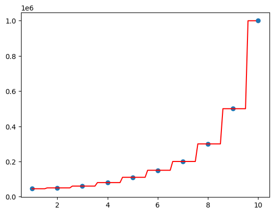
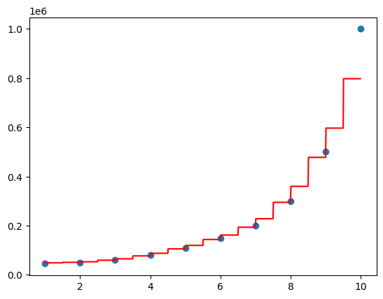
Decision tree regression will split according to features and assign an average value to a particular range
Random Forest Regression#
Decision Trees tend to overfit the model. What random forest does is creates many different trees with random variables, and the end outcome is averaged across all the trees. This avoids overfitting and gives an accurate model
import pandas as pd
import matplotlib.pyplot as plt
import numpy as np

df = pd.read_csv('Position_Salaries.csv')
X = df.iloc[:, 1:2]   # Using 1:2 as indices will give us np array of dim (10, 1)
y = df.iloc[:, 2]

df.head()
| Position | Level | Salary | |
|---|---|---|---|
| 0 | Business Analyst | 1 | 45000 |
| 1 | Junior Consultant | 2 | 50000 |
| 2 | Senior Consultant | 3 | 60000 |
| 3 | Manager | 4 | 80000 |
| 4 | Country Manager | 5 | 110000 |
from sklearn.ensemble import RandomForestRegressor
regressor = RandomForestRegressor(n_estimators=1000, random_state=0).fit(X, y)
plt.scatter(X, y)
X_grid = np.arange(min(X.values), max(X.values), 0.01).reshape(-1, 1)
plt.plot(X_grid, regressor.predict(X_grid), color='r')
plt.show()
/var/folders/7m/04ssj6n96q984_6wsnr60dg00000gn/T/ipykernel_92876/710121559.py:2: DeprecationWarning: Conversion of an array with ndim > 0 to a scalar is deprecated, and will error in future. Ensure you extract a single element from your array before performing this operation. (Deprecated NumPy 1.25.)
  X_grid = np.arange(min(X.values), max(X.values), 0.01).reshape(-1, 1)
/opt/homebrew/Caskroom/miniconda/base/envs/ml-notes/lib/python3.12/site-packages/sklearn/base.py:493: UserWarning: X does not have valid feature names, but RandomForestRegressor was fitted with feature names
  warnings.warn(