LoRA (Low Rank Adaptation of Large Language Models)#
Before diving into LoRA, it’s essential to grasp the concept of Matrix Decomposition.
Matrix Decomposition involves breaking down large matrices into smaller ones while retaining as much information as possible. This process is particularly useful when dealing with large rank matrices, such as those in Large Language Models (LLMs). By removing highly correlated features (or repeated sets of information), we can compress the data into smaller matrices.
For example, in images, multiple pixels that are close to each other may be highly correlated. These highly correlated matrices are called Low-Rank Matrices because essential information is present only in fewer rows or columns…
The essence of Low-Rank Matrix Factorization lies in decomposing a large matrix into a product of two or more smaller, simpler matrices with a lower rank.
The goal of Low-Rank Matrix Factorization is to approximate a high-dimensional matrix M and \(B\) as a product of two smaller matrices A and B
Mathematically, this can be expressed as M ≈ A x B, where M is an m x n matrix, A is an m x k matrix, and B is a k × n matrix, with k (the rank) being much smaller than both m and n.
The purpose of this decomposition is to reduce the dimensionality of the matrix while retaining its primary features and structure.
For a detailed explanation, refer to the blog post below:
Matrix Decomposition Series: Low-Rank Matrix Factorization
Training Language Models: Existing Approaches#
When training a language model on your dataset, you typically have a few options:
Full Fine-Tuning: Retraining all model parameters becomes less feasible as model size increases. For example, fine-tuning GPT-3 with 175 billion parameters for multiple instances is prohibitively expensive.
Fine-Tuning with Additional Layers: Adding trainable layers on top of a pre-trained model, known as adapter layers, introduces additional latency and doesn’t integrate well with distributed processing, as adapter layers must be inferred sequentially.
Prompt Tuning:
Hard Prompt Tuning: Involves creating handcrafted text prompts with discrete input tokens, which is labor-intensive.
Soft Prompt Tuning: Uses learnable tensors concatenated with input embeddings optimized for a dataset. However, these “virtual tokens” are not human-readable, as they don’t match real-word embeddings.
Introducing LoRA: Low-Rank Adaptation#
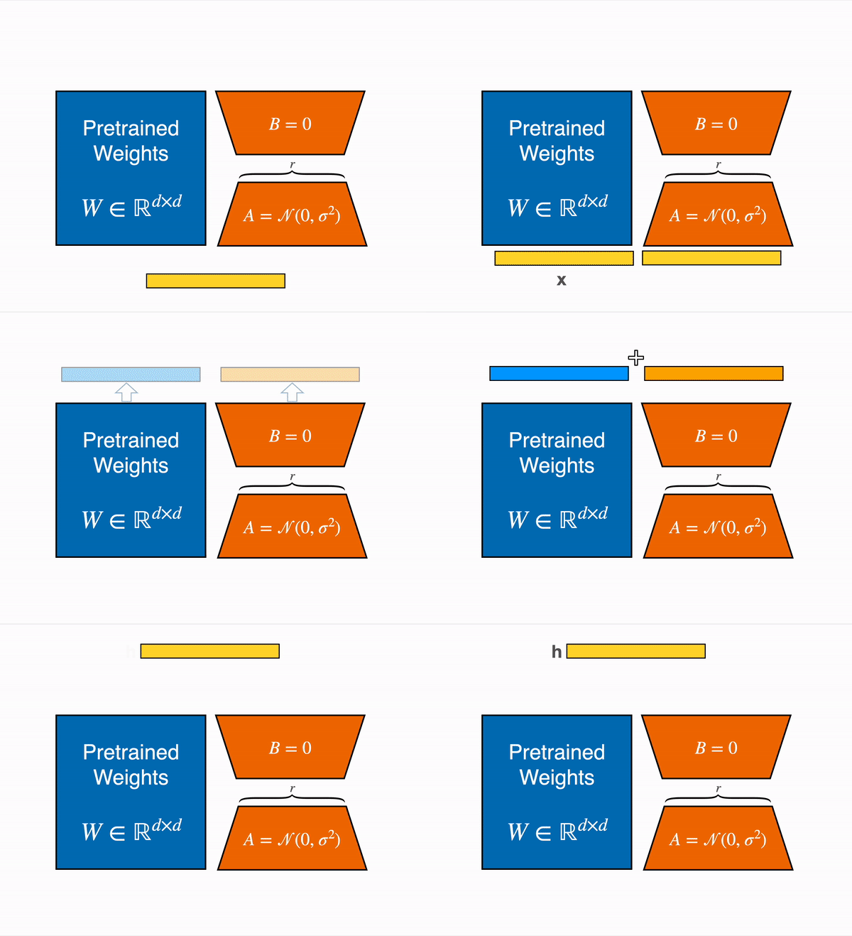
Fine-tuning large models like GPT-3 by retraining all parameters is both computationally and memory expensive. Low-Rank Adaptation (LoRA) offers a solution by freezing pre-trained model weights and injecting trainable rank decomposition matrices into each layer of the Transformer architecture. This significantly reduces the number of trainable parameters and GPU memory requirements, while maintaining or even improving model performance, thus accelerating fine-tuning while consuming less memory.
A neural network contains many dense layers which perform matrix multiplication. The weight matrices in these layers typically have full-rank. When adapting to a specific task, the pre-trained language models have a low “instrisic dimension” and can still learn efficiently despite a random projection to a smaller subspace.
Inspired by this, there is a hypothesis that the updates to the weights also have a low “intrinsic rank” during adaptation. For a pre-trained weight matrix \(W_0 ∈ W_0 \in \mathbb{R}^{d \times k}\) , we constrain its update by representing the latter with a low-rank decomposition \(W_0 + \Delta W = W_0 + BA\), where \(B \in \mathbb{R}^{d \times r}, A \in \mathbb{R}^{r \times k}\) , and the rank r \(r \leq \min(d, k)\). During training, \(W_{0}\) is frozen and does not receive gradient updates, while A and B contain trainable parameters. Note both \(W_{0}\) and \(∆W = BA\) are multiplied with the same input, and their respective output vectors are summed coordinate-wise. For \(h = W_{0}x\), our modified forward pass yields: $\(h = W_{0}x + ∆W x = W_{0}x + BAx\)\( At the beginning of training \)A\( is initialised with random Gaussian initialisation, while \)B$ is initialised with 0.
LoRA represents the weight updates ΔW with two smaller matrices (called update matrices) through low-rank decomposition. These new matrices can be trained to adapt to new data while keeping the overall number of parameters low. The original weight matrix remains frozen and doesn’t receive further updates. To produce the final results, the original and adapted weights are combined. Alternatively, you can merge the adapter weights with the base model to eliminate inference latency.

Which weight matrices should be adapted#
Based on the findings mentioned in the paper, adapting LoRA to both \(W_{}q\) and \(W_{v}\) together yields the best downstream performance.
What should be the optimal rank \(r\)#
LoRA already performs competitively with a very small r (more so for \({Wq, Wv}\) than just \(Wq\)). This suggests the update matrix \(∆W\) could have a very small “intrinsic rank”. Small ranks like \(r=1\) and \(r=2\) can be surprisingly effective.
Correlation between \(ΔW\) & \(W\)#
∆W has a stronger correlation with \(W\) compared to a random matrix,
Indicating that ∆W amplifies some features that are already in \(W\).
Second, instead of repeating the top singular directions of \(W\), \(∆W\) only amplifies directions that are not emphasized in \(W\).
Third, the amplification factor is rather huge: 21.5 ≈ 6.91/0.32 for r = 4.
This suggests that the low-rank adaptation matrix potentially amplifies the important features for specific downstream tasks that were learned but not emphasized in the general pre-training model.
Advantages of LoRA#
Efficiency: LoRA drastically reduces the number of trainable parameters.
Flexibility: The original pretrained weights are kept frozen, allowing multiple lightweight and portable LoRA models to be built for various downstream tasks.
Compatibility: LoRA is orthogonal to other parameter-efficient methods and can be combined with many of them.
Performance: Models fine-tuned using LoRA perform comparably to fully fine-tuned models.
In principle, LoRA can be applied to any subset of weight matrices in a neural network to reduce the number of trainable parameters. However, for simplicity and further parameter efficiency, LoRA is typically only applied to the attention blocks in Transformer models. The resulting number of trainable parameters in a LoRA model depends on the size of the update matrices, which is determined mainly by the rank r and the shape of the original weight matrix.

Comments
comments powered by Disqus